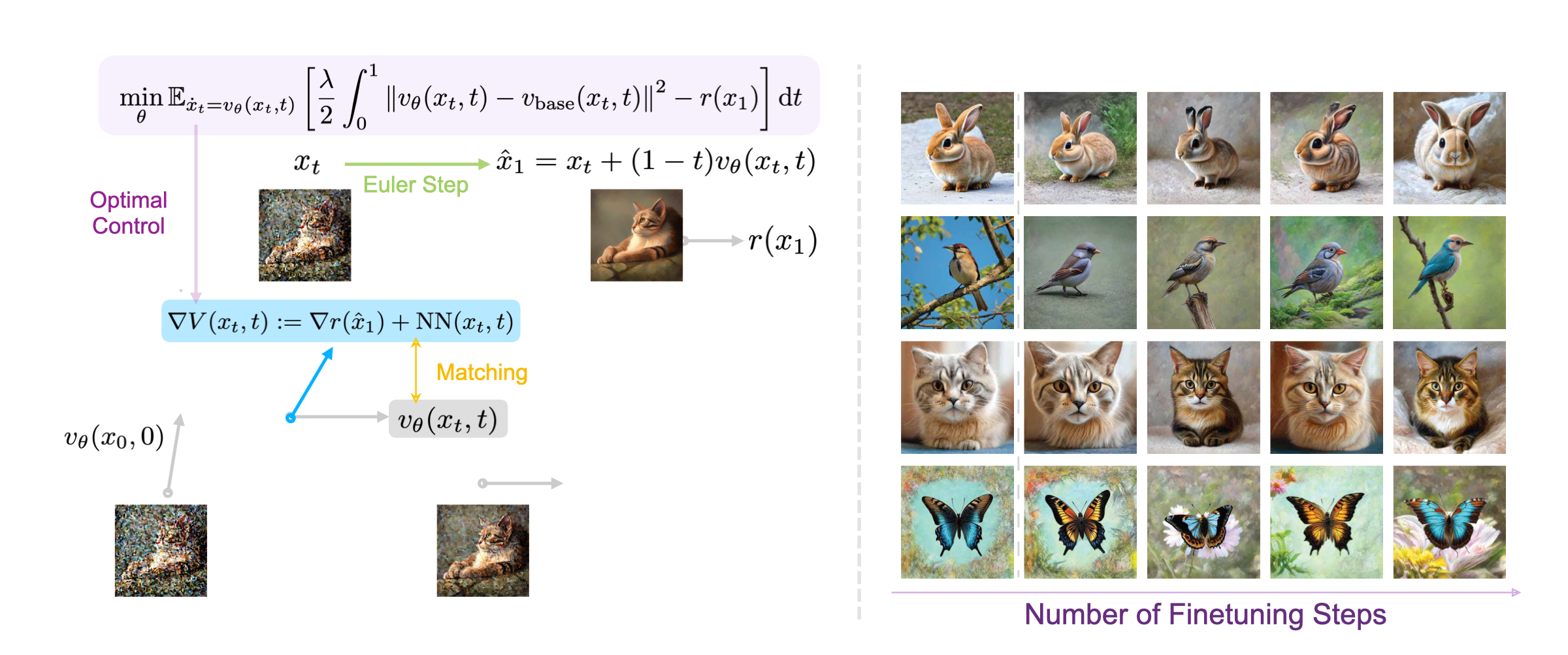
VGG-Flow starts from an optimal-control objective, derives
value-gradient matching from the HJB equation, then trains a
value-gradient model and flow model jointly with three losses.
0. Flow Matching Preliminaries
A flow matching model starts from Gaussian noise and maps it to
a data sample by integrating a learned ODE velocity field.
\[
x_0 \sim \mathcal{N}(0, I), \qquad \dot{x}_t =
v_{\theta}(x_t,t), \quad t \in [0,1], \qquad x_1 = x(t=1).
\]
VGG-Flow finetunes this velocity field while preserving the base
prior through a control-style regularization.
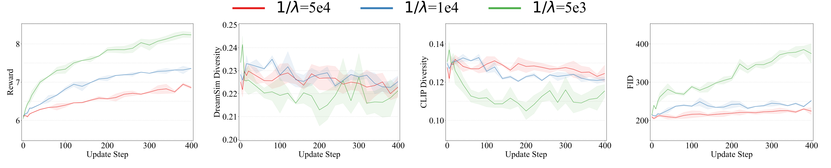
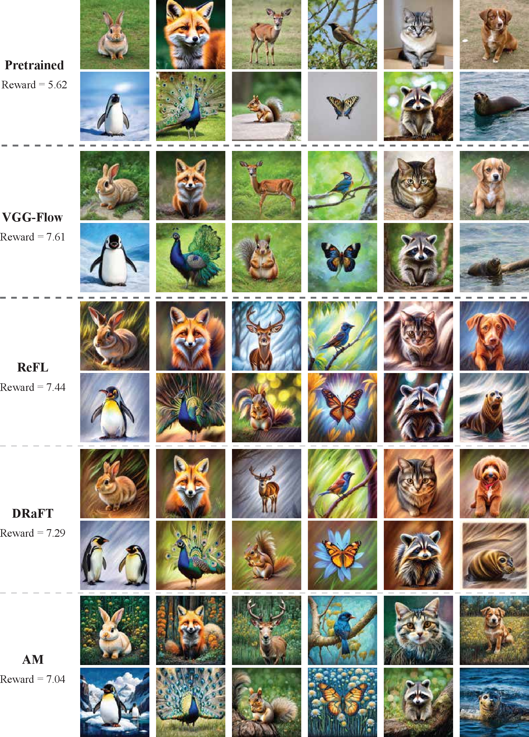
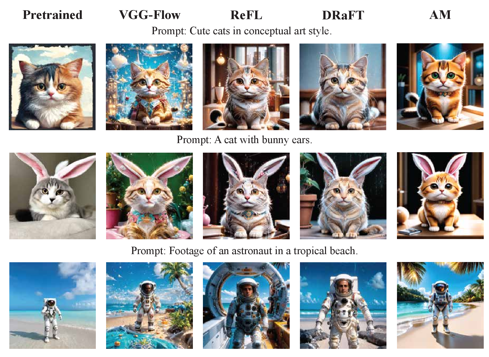
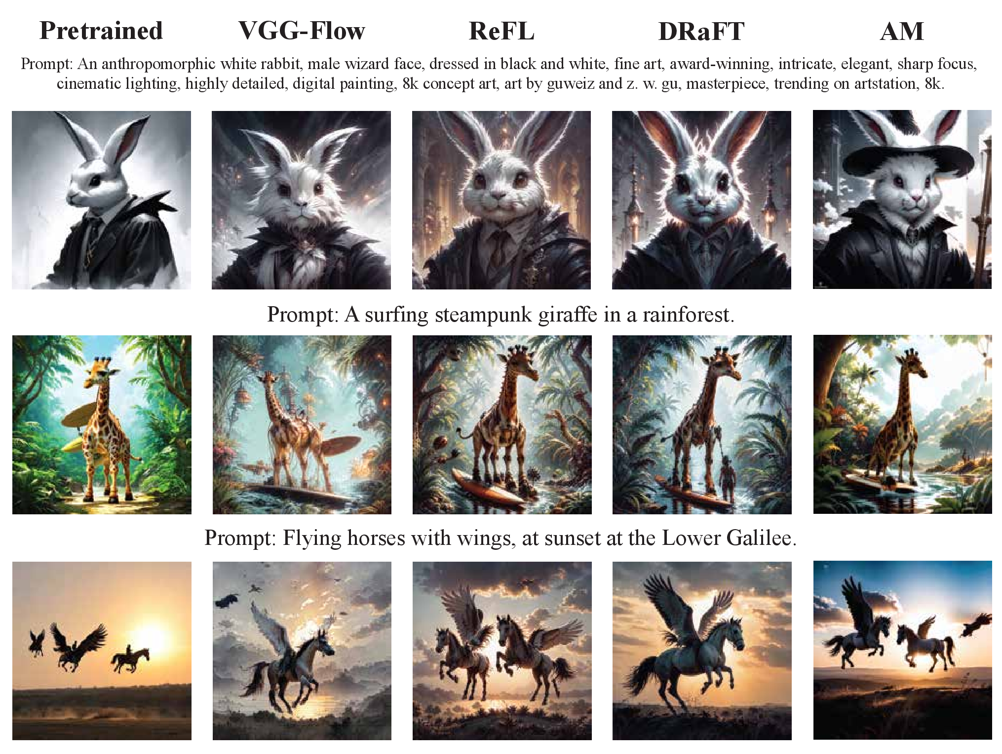
1. Alignment Objective
Finetune a base velocity field with a reward objective plus a
quadratic control cost that keeps the model close to the
pretrained prior.
\[
\min_{\theta}\,\mathbb{E}_{x_0\sim p_0,\dot{x}_t=v_{\theta}(x_t,t)}
\left[\frac{\lambda}{2}\int_{0}^{1}\left\lVert
\tilde{v}_{\theta}(x_t,t)\right\rVert^2\,dt-r(x_1)\right],\quad
v_{\theta}(x_t,t)\triangleq
v_{\mathrm{base}}(x_t,t)+\tilde{v}_{\theta}(x_t,t).
\]
2. HJB Condition and Control Law
Applying HJB yields the optimal residual velocity and links it
directly to the value-function gradient.
\[
\partial_tV(x,t)+\min_{\tilde{v}}\left[\nabla V(x,t)\cdot
\big(v_{\mathrm{base}}(x,t)+\tilde{v}(x,t)\big)
+\frac{\lambda}{2}\|\tilde{v}(x,t)\|^2\right]=0.
\]
Direct HJB result: Value Gradient Matching
\[
\tilde{v}^{\star}(x,t)=-\frac{1}{\lambda}\nabla V(x,t).
\]
Direct HJB result: Value Consistency
\[
\partial_tV(x,t)=\frac{1}{2\lambda}\|\nabla V(x,t)\|^2-\nabla
V(x,t)\cdot v_{\mathrm{base}}(x,t).
\]
3. Value-Gradient Parameterization
The value gradient is parameterized with a forward-looking term:
reward gradient from a one-step Euler prediction plus a learnable
residual.
\[
g_{\phi}(x,t)\triangleq\nabla V_{\phi}(x,t).
\]
\[
g_{\phi}(x,t)\triangleq-\eta_t\cdot\operatorname{stop\mbox{-}gradient}
\left(\nabla_{x_t}r\!\left(\hat{x}_1(x_t,t)\right)\right)+\nu_{\phi}(x_t,t).
\]
4. Training Losses
The final training objective combines matching loss, consistency
loss, and boundary loss.
\[
\mathcal{L}_{\mathrm{matching}}(\theta)=
\mathbb{E}_{x_0\sim\mathcal{N}(0,I),\dot{x}_t=v(x_t,t)}
\left\lVert\tilde{v}_{\theta}(x_t,t)+\beta g_{\phi}(x_t,t)\right\rVert^2.
\]
\[
\mathcal{L}_{\mathrm{consistency}}(\phi)=
\mathbb{E}_{x_0\sim\mathcal{N}(0,I),\dot{x}_t=v(x_t,t)}
\left\lVert\frac{\partial}{\partial t}g_{\phi}
+[\nabla g_{\phi}]^{\top}(v_{\mathrm{base}}-\beta g_{\phi})
+[\nabla v_{\mathrm{base}}]^{\top}g_{\phi}\right\rVert^2.
\]
\[
\mathcal{L}_{\mathrm{boundary}}(\phi)=
\mathbb{E}_{x_0\sim\mathcal{N}(0,I),\dot{x}_t=v(x_t,t)}
\left\lVert g_{\phi}(x_1,1)+\nabla r(x_1)\right\rVert^2.
\]
\[
\mathcal{L}_{\mathrm{total}}(\theta,\phi)=
\mathcal{L}_{\mathrm{matching}}(\theta)+
\mathcal{L}_{\mathrm{consistency}}(\phi)+
\alpha\mathcal{L}_{\mathrm{boundary}}(\phi).
\]